Building a Powerful Content Moderation Classifier with Scikit-Learn and LightGBM

Content moderation is a critical task for any online platform. The goal is to automatically identify and flag content that violates community guidelines, covering categories like hate speech, harassment, or self-harm. While large language models (LLMs) have become popular, traditional machine learning models remain powerful, efficient, and highly effective, especially when enhanced with smart feature engineering.

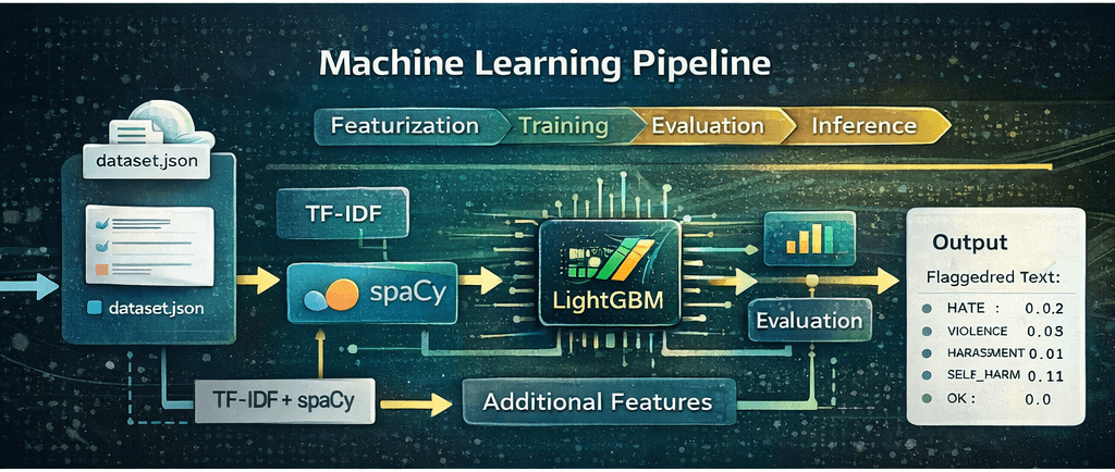
In this blog, we'll walk through a step-by-step guide to building a robust multi-label text classifier for content moderation. We will:

1. Start with a strong baseline model using TF-IDF and a LightGBM classifier.
2. Develop a clean inference pipeline to use our trained model.
3. Enhance our model by engineering contextual features using spaCy for lemmatization and sentiment analysis.
4. Combine all features using Scikit-Learn's FeatureUnion to train a final, more powerful classifier.

Let's get started! 🚀

Installing and Importing Libraries

First, let's install the necessary Python libraries. We'll be using scikit-learn for our modeling pipeline, lightgbm as our powerful classifier, pandas for data manipulation, and spacy for advanced text processing.

!pip install scikit-learn pandas lightgbm numpy spacy -q
!python -m spacy download en_core_web_sm -q  

import io
import json
import warnings

import joblib
import nltk
import numpy as np
import pandas as pd
import spacy
from google.colab import files
from lightgbm import LGBMRegressor
from nltk.sentiment.vader import SentimentIntensityAnalyzer
from sklearn.base import BaseEstimator, TransformerMixin
from sklearn.feature_extraction.text import TfidfVectorizer
from sklearn.metrics import f1_score, mean_squared_error, roc_auc_score
from sklearn.model_selection import train_test_split
from sklearn.multioutput import MultiOutputRegressor
from sklearn.pipeline import FeatureUnion, Pipeline
from sklearn.preprocessing import StandardScaler

warnings.filterwarnings('ignore')

try:
    nltk.data.find("sentiment/vader_lexicon.zip")
except Exception:
    nltk.download("vader_lexicon")

Loading the Dataset

Our dataset is a JSON file where each entry contains a piece of text and a corresponding dictionary of labels. For this multi-label problem, each text can be associated with one, multiple, or no labels.

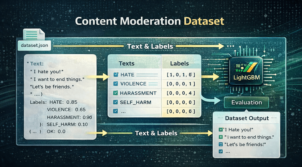
Let's upload our dataset and inspect its structure.

# Download the JSON file from Google Drive using gdown
!pip install gdown -q
!gdown 1axUt7M0n2wiWFleWqXo49Yj6x2U9YDXw -O data.json

# Load the JSON data from the downloaded file
with open('data.json', 'r') as f:
    data = json.load(f)

print("Successfully loaded data.json!")
print("\nHere's a sample from the dataset:")
print(json.dumps(data[0], indent=2))

Downloading...
From: https://drive.google.com/uc?id=1axUt7M0n2wiWFleWqXo49Yj6x2U9YDXw
To: /content/data.json
100% 7.96M/7.96M [00:00<00:00, 53.7MB/s]
Successfully loaded data.json!

Here's a sample from the dataset:
{
  "text": "I'm a teenager and I'm thinking about suicide. I haven't attempted it yet, but I'm thinking about it a lot. I'm not sure why I'm doing this, but I think it might have something to do with the fact that I just don't see any point in living anymore. I'm not happy and I don't think things will ever get better.\n\nI've been thinking about ways to do it and the one that seems the most painless is to just drive my car into a parking garage and put it in neutral and let it crash into the wall. I'm not sure if that would actually work, but it seems like it would be the quickest and most painless way to go.",
  "labels": {
    "SEXUAL": 0.0,
    "HATE": 0.0,
    "VIOLENCE": 0.0,
    "HARASSMENT": 0.0,
    "SELF_HARM": 1.0,
    "SEXUAL_MINORS": 0.0,
    "HATE_THREATENING": 0.0,
    "VIOLENCE_GRAPHIC": 0.0,
    "OK": 0.0
  }
}

Next, we'll define a helper function to process this list of dictionaries into separate lists for texts, labels, and the names of the label columns.

def load_data(data: list[dict]):
    """
    Loads and prepares data from the list of dictionaries.
    """
    label_names = sorted(data[0]["labels"].keys())
    texts = [item["text"] for item in data]
    labels = np.array([[float(item["labels"].get(label, 0.0)) for label in label_names] for item in data])
    return texts, labels, label_names

Defining Our Evaluation Method

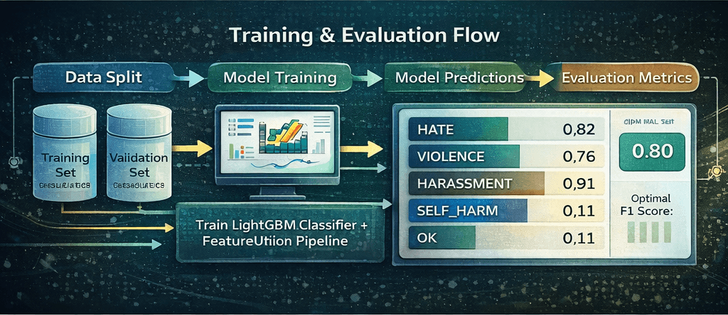
Before we start training, it's crucial to decide how we'll measure success. Since this is a multi-label classification problem treated as regression (predicting scores from 0 to 1), we'll use a few key metrics:

1. Mean Squared Error (MSE): Measures how wrong your model's predictions are, on average. Lower is better.
2. ROC AUC (micro): Evaluates how good your model is at telling things apart. It checks how well the model can distinguish between groups. Higher is better.
3. F1 Score (micro): A single number that balances two important qualities: precision and recall.
4. Precision is about not making false positive mistakes.
5. Recall is about not missing any positive cases.

This function will help us evaluate our models consistently.

def evaluate_predictions(y_true, y_pred_probs):
    """
    Evaluates predictions and finds the optimal F1 score by searching across thresholds.
    """
    y_true_binary = (y_true >= 0.5).astype(int)

    # Find best F1 score by iterating through potential thresholds
    thresholds = np.arange(0.1, 0.9, 0.01)
    best_f1 = 0
    best_threshold = 0.5
    for threshold in thresholds:
        f1 = f1_score(y_true_binary, (y_pred_probs >= threshold).astype(int), average="micro", zero_division=0)
        if f1 > best_f1:
            best_f1 = f1
            best_threshold = threshold

    # Calculate other metrics
    mse = mean_squared_error(y_true, y_pred_probs)
    roc_auc = roc_auc_score(y_true_binary, y_pred_probs, average="micro")

    metrics = {
        'mse': mse,
        'roc_auc_micro': roc_auc,
        'f1_micro': best_f1,
        'optimal_threshold': best_threshold,
    }
    return metrics

You might have observed an extra step in this method: determining the optimal threshold for our F1 score. The F1 score itself is evaluated on binary outcomes (0 or 1). Since our model outputs continuous probabilities (floating-point numbers between 0.0 and 1.0), we need a threshold to convert these probabilities into discrete binary labels. This threshold dictates whether a text is classified as related (1) or not related (0).

Selecting the threshold that maximizes the F1 score is important. In practical applications, this allows us to understand the specific confidence level required to flag a text as relevant.

Baseline Model: TF-IDF + LightGBM

Let's create our first model. We'll use a classic but powerful combination:

1. TfidfVectorizer: This converts raw text into a matrix of numerical features based on word frequency, adjusted for how common words are across all texts. It's a fantastic starting point for text classification.
2. MultiOutputRegressor: This is a Scikit-Learn wrapper that allows us to use any regressor (like LightGBM) for multi-label tasks. It works by training one separate regressor for each of our target labels (e.g., one for 'HATE', one for 'VIOLENCE', etc.).
3. LGBMRegressor: LightGBM is a state-of-the-art gradient boosting framework known for its speed and accuracy.

We'll package these steps into a Pipeline to keep our workflow clean and reproducible.

# Load and split the data into training and validation sets
texts, labels, label_names = load_data(data)
train_texts, val_texts, train_labels, val_labels = train_test_split(
    texts, labels, test_size=0.2, random_state=42
)

# Define the baseline model pipeline
baseline_pipeline = Pipeline(
    [
        (
            "vectorizer",
            TfidfVectorizer(
                max_features=20000,
                ngram_range=(1, 2),
                sublinear_tf=True,
                stop_words="english",
            ),
        ),
        (
            "classifier",
            MultiOutputRegressor(
                LGBMRegressor(random_state=42),
                n_jobs=-1, # Use all available CPU cores
            ),
        ),
    ]
)

# Train the model
print("Training baseline ML pipeline...")
baseline_pipeline.fit(train_texts, train_labels)
print("Training complete.")

# Make predictions and clip results to the valid [0, 1] range
val_predictions = baseline_pipeline.predict(val_texts)
np.clip(val_predictions, 0, 1, out=val_predictions)

# Evaluate the model
print("\nEvaluating model performance...")
metrics = evaluate_predictions(val_labels, val_predictions)

print("\nBaseline ML Model Metrics:")
for key, value in metrics.items():
    print(f"- {key}: {value:.4f}")

# Save the trained pipeline and labels for later use
joblib.dump(baseline_pipeline, 'baseline_ml_pipeline.joblib')
with open('labels.json', 'w') as f:
    json.dump(label_names, f)

Training baseline ML pipeline...
Training complete.

Evaluating model performance...

Baseline ML Model Metrics:
- mse: 0.0565
- roc_auc_micro: 0.8923
- f1_micro: 0.6978
- optimal_threshold: 0.3400

With an F1 score of ~0.70, our baseline is already quite capable! Now, let's build a simple class to make it easy to perform inference on new text.

Making Predictions (Inference)

To make our model easy to use, we'll create a Predictor class. This class will load our saved pipeline and labels.json files and provide a clean .predict() method that takes a list of texts and returns formatted predictions.

class Predictor:
    """
    A class to load a trained scikit-learn pipeline and make predictions.
    """
    def __init__(self, model_path: str, labels_path: str):
        print(f"Loading model from {model_path}...")
        self.pipeline = joblib.load(model_path)

        print(f"Loading labels from {labels_path}...")
        with open(labels_path, 'r') as f:
            self.label_names = json.load(f)

    def predict(self, texts: list[str]) -> list[dict]:
        """
        Performs inference on a list of texts.
        """
        # The pipeline handles both vectorization and prediction
        results = self.pipeline.predict(texts)
        np.clip(results, 0, 1, out=results)

        # Format the output into a list of dictionaries
        predictions = []
        for i, text in enumerate(texts):
            label_scores = {self.label_names[j]: score for j, score in enumerate(results[i])}
            predictions.append({"text": text, "scores": label_scores})

        return predictions

# Define the paths to our saved model artifacts
MODEL_PATH = 'baseline_ml_pipeline.joblib'
LABELS_PATH = 'labels.json'

# List of example texts to classify
texts_to_predict = [
    "Those people from Hogwarts are all ugly and stupid",
    "Can anyone recommend a good book to read?",
    "That is definetely the worst dress I've ever seem, you look horrible, ugly, horrendous.",
    "DUMBASS!! You don't even know that?"
]

# Initialize the predictor and get predictions
predictor = Predictor(model_path=MODEL_PATH, labels_path=LABELS_PATH)
predictions = predictor.predict(texts_to_predict)

# Print the results nicely
for pred in predictions:
    print(f'\nText: "{pred["text"]}"')
    print("Scores:")
    sorted_scores = sorted(pred["scores"].items(), key=lambda item: item[1], reverse=True)
    for label, score in sorted_scores:
        print(f"  - {label}: {score:.4f}")

Loading model from baseline_ml_pipeline.joblib...
Loading labels from labels.json...

Text: "Those people from Hogwarts are all ugly and stupid"
Scores:
  - HATE: 0.7541
  - OK: 0.3640
  - HARASSMENT: 0.2945
  - HATE_THREATENING: 0.2600
  - VIOLENCE: 0.1293
  - SEXUAL_MINORS: 0.0153
  - VIOLENCE_GRAPHIC: 0.0094
  - SELF_HARM: 0.0000
  - SEXUAL: 0.0000

Text: "Can anyone recommend a good book to read?"
Scores:
  - OK: 0.5923
  - HATE: 0.2679
  - HARASSMENT: 0.2195
  - HATE_THREATENING: 0.2062
  - SEXUAL: 0.0965
  - VIOLENCE: 0.0637
  - SEXUAL_MINORS: 0.0494
  - VIOLENCE_GRAPHIC: 0.0391
  - SELF_HARM: 0.0000

Text: "That is definetely the worst dress I've ever seem, you look horrible, ugly, horrendous."
Scores:
  - OK: 0.5261
  - HATE: 0.5161
  - HARASSMENT: 0.3939
  - HATE_THREATENING: 0.2042
  - SEXUAL_MINORS: 0.0843
  - VIOLENCE: 0.0674
  - VIOLENCE_GRAPHIC: 0.0176
  - SEXUAL: 0.0090
  - SELF_HARM: 0.0000

Text: "DUMBASS!! You don't even know that?"
Scores:
  - OK: 0.5174
  - HATE: 0.3063
  - HARASSMENT: 0.1819
  - HATE_THREATENING: 0.1547
  - VIOLENCE: 0.0325
  - SEXUAL: 0.0152
  - VIOLENCE_GRAPHIC: 0.0028
  - SELF_HARM: 0.0000
  - SEXUAL_MINORS: 0.0000

The baseline model performs acceptably on the first two examples. However, it struggles with the latter two, incorrectly assigning the highest score to the "OK" class when "HATE" should have been ranked higher.

The primary issue is that the model relies solely on word count, failing to grasp the underlying context.

This is where feature engineering becomes crucial. Can we introduce additional contextual signals to enable our model to make more accurate distinctions?

Enhanced Model: Adding Context with Feature Engineering

TF-IDF is great, but it only looks at word frequencies. To improve our model, we can add features that capture more about the meaning and style of the text. We will create two custom transformers to do this:

1. SpacyLemmatizer: Instead of just using words as they are, lemmatization reduces words to their root form (or 'lemma'). For example, 'cutting', 'cut', and 'cuts' all become 'cut'. This helps the model generalize better by consolidating related words into a single feature. We'll integrate this directly into our TfidfVectorizer.
2. FeatureEngineer: This transformer will create additional numerical features for each text:
   1. Sentiment Scores: Using NLTK's VADER, we'll get positive, negative, and compound sentiment scores. A very negative score might be a strong indicator of hate speech or harassment.
   2. Text Statistics: Simple features like text length and the ratio of uppercase letters can be surprisingly effective. For example, texts with many capital letters ('SHOUTING') often signal aggression.

class SpacyLemmatizer:
    """
    A callable class for spaCy lemmatization inside TfidfVectorizer.
    This approach is memory-efficient as it loads the spaCy model only once.
    """
    def __init__(self):
        self.nlp = spacy.load("en_core_web_sm", disable=["parser", "ner"])
        # Disabling 'tok2vec' can prevent potential multiprocessing errors with scikit-learn
        if self.nlp.has_pipe("tok2vec"):
             self.nlp.disable_pipe("tok2vec")

    def __call__(self, doc):
        # Process the document and return a list of lemmas
        return [
            token.lemma_ for token in self.nlp(doc)
            if not token.is_punct and not token.is_stop
        ]

class FeatureEngineer(BaseEstimator, TransformerMixin):
    """
    Custom transformer to create sentiment and statistical features.
    """
    def __init__(self):
        self.sia = SentimentIntensityAnalyzer()

    def fit(self, X, y=None):
        return self

    def transform(self, X):
        features = []
        for text in X:
            # 1. Sentiment scores
            sentiment = self.sia.polarity_scores(text)

            # 2. Text statistics
            text_len = len(text)
            upper_ratio = sum(1 for c in text if c.isupper()) / text_len if text_len > 0 else 0

            # Combine all features for this text
            features.append([
                sentiment['pos'],
                sentiment['neg'],
                sentiment['compound'],
                text_len,
                upper_ratio
            ])
        return np.array(features)

Combining Features with FeatureUnion

Now, we'll use FeatureUnion to combine the outputs of our lemmatized TF-IDF vectorizer and our custom FeatureEngineer. This powerful tool runs both transformers in parallel and concatenates their resulting feature matrices, giving our final classifier a richer, more diverse set of inputs to learn from.

# Define the enhanced model pipeline
enhanced_pipeline = Pipeline(
    [
        (
            "features",
            FeatureUnion(
                [
                    (
                        "tfidf_lemmatized",
                        TfidfVectorizer(
                            tokenizer=SpacyLemmatizer(),
                            max_features=12000,
                            ngram_range=(1, 2),
                        ),
                    ),
                    (
                        "custom_features",
                        Pipeline([
                            ('engineer', FeatureEngineer()),
                            ('scaler', StandardScaler())
                        ])
                    ),
                ]
            ),
        ),
        ("classifier", MultiOutputRegressor(LGBMRegressor(random_state=42), n_jobs=-1)),
    ]
)

# Train the model
print("Training enhanced ML pipeline...")
enhanced_pipeline.fit(train_texts, train_labels)
print("Training complete.")

# Make predictions and clip results
val_predictions_enhanced = enhanced_pipeline.predict(val_texts)
np.clip(val_predictions_enhanced, 0, 1, out=val_predictions_enhanced)

# Evaluate the model
print("\nEvaluating enhanced model performance...")
metrics_enhanced = evaluate_predictions(val_labels, val_predictions_enhanced)

print("\nEnhanced ML Model Metrics:")
for key, value in metrics_enhanced.items():
    print(f"- {key}: {value:.4f}")

# Save the new enhanced model
joblib.dump(enhanced_pipeline, 'enhanced_ml_pipeline.joblib')

Training enhanced ML pipeline...
Training complete.

Evaluating enhanced model performance...

Enhanced ML Model Metrics:
- mse: 0.0567
- roc_auc_micro: 0.8924
- f1_micro: 0.6948
- optimal_threshold: 0.3500
['enhanced_ml_pipeline.joblib']

Our new model shows similar metrics, but that doesn't necessarily mean there hasn't been improvement. Our current dataset may not contain many examples that specifically benefit from our new features, such as sentiment analysis or the use of uppercase text. However, real-world scenarios are likely to include such instances.

# Initialize the predictor with the new enhanced model
predictor_enhanced = Predictor(model_path='enhanced_ml_pipeline.joblib', labels_path=LABELS_PATH)

# Get predictions for the same list of texts
predictions_enhanced = predictor_enhanced.predict(texts_to_predict)

# Print the results
print("--- Predictions from Enhanced Model ---")
for pred in predictions_enhanced:
    print(f'\nText: "{pred["text"]}"')
    print("Scores:")
    sorted_scores = sorted(pred["scores"].items(), key=lambda item: item[1], reverse=True)
    for label, score in sorted_scores:
        print(f"  - {label}: {score:.4f}")

Loading model from enhanced_ml_pipeline.joblib...
Loading labels from labels.json...
--- Predictions from Enhanced Model ---

Text: "Those people from Hogwarts are all ugly and stupid"
Scores:
  - HATE: 0.8595
  - HATE_THREATENING: 0.4517
  - HARASSMENT: 0.4337
  - VIOLENCE: 0.2091
  - OK: 0.2065
  - VIOLENCE_GRAPHIC: 0.0436
  - SEXUAL_MINORS: 0.0430
  - SELF_HARM: 0.0089
  - SEXUAL: 0.0000

Text: "Can anyone recommend a good book to read?"
Scores:
  - OK: 0.5895
  - HATE: 0.2803
  - HARASSMENT: 0.2751
  - HATE_THREATENING: 0.2245
  - SEXUAL: 0.1039
  - VIOLENCE: 0.0241
  - SEXUAL_MINORS: 0.0216
  - VIOLENCE_GRAPHIC: 0.0144
  - SELF_HARM: 0.0000

Text: "That is definetely the worst dress I've ever seem, you look horrible, ugly, horrendous."
Scores:
  - HATE: 0.6806
  - HARASSMENT: 0.4879
  - HATE_THREATENING: 0.4391
  - OK: 0.2588
  - VIOLENCE: 0.2521
  - VIOLENCE_GRAPHIC: 0.0969
  - SEXUAL_MINORS: 0.0853
  - SEXUAL: 0.0472
  - SELF_HARM: 0.0083

Text: "DUMBASS!! You don't even know that?"
Scores:
  - HATE: 0.5723
  - HATE_THREATENING: 0.4475
  - HARASSMENT: 0.3642
  - OK: 0.2462
  - SEXUAL_MINORS: 0.1585
  - VIOLENCE: 0.1323
  - SEXUAL: 0.0532
  - VIOLENCE_GRAPHIC: 0.0513
  - SELF_HARM: 0.0046

Adding features like sentiment analysis and text statistics provided the model with crucial context beyond simple words, resulting in a much more accurate and reliable classifier.

Conclusion & Key Takeaways

Our enhanced model now correctly identifies the hate text with higher confidence. This is a direct result of adding features that provided deeper context beyond simple word counts.

Traditional ML models are remarkably efficient, boasting low resource consumption and fast training times. This makes them an accessible and cost-effective choice for many real-world applications.

However, their main limitation is that they do not tend to generalize as well as their larger counterparts. Their success is directly tied to the quality of the features you provide. To unlock their potential, you must become a domain expert for your data. In our content moderation example, we didn't just use raw text; we cleverly engineered features like sentiment scores and uppercase ratios because we hypothesized they were strong signals for toxicity. This targeted approach made all the difference.

If you have a specific use-case, take the time to understand the nuances of your own data. By engineering features that reflect those unique patterns, you can build a highly effective and efficient model that performs exceptionally well for your specific needs.

In the next blog post we will be covering Transformers based multi-label text classification.