

OpenCV Edge, Shape, and Feature Detection
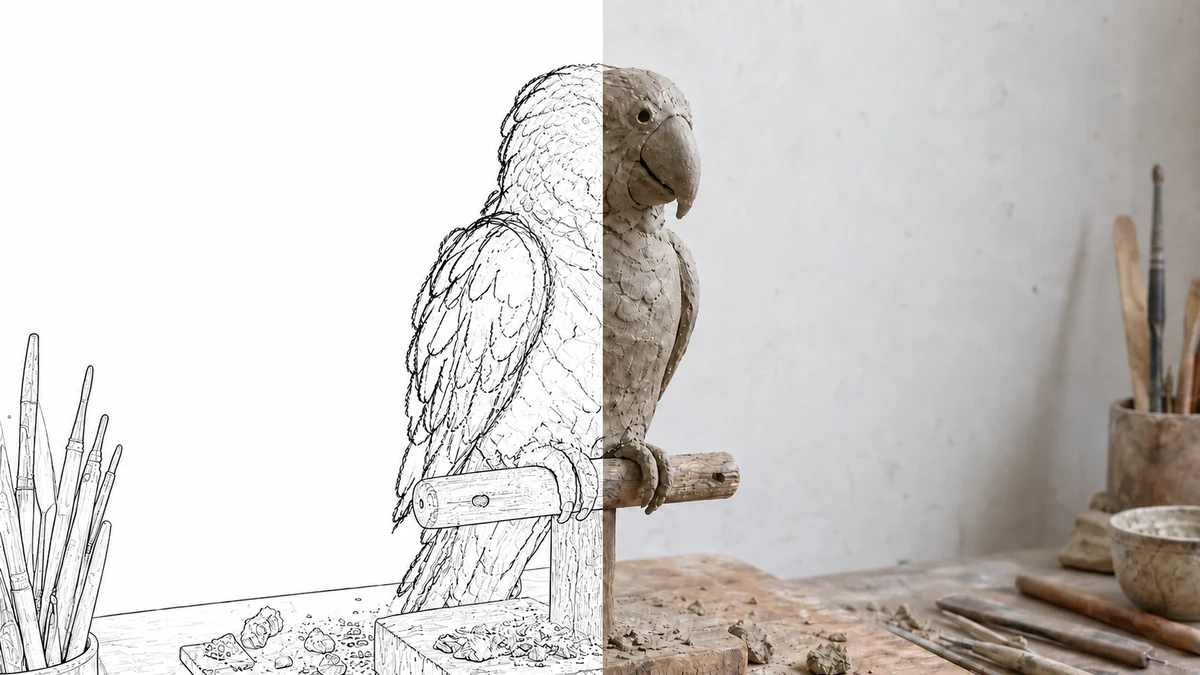
Once an image is cleaned up and segmented, the next step is to find structure in it: edges, outlines, lines, circles, and repeated patterns. These features drive document scanners, inspection systems, lane detection, and many other computer vision applications, and they are often the fastest way to solve a well-controlled problem without training a model.
Part 1 covers edge detection, contour detection, and morphological operations. Part 2 covers pattern recognition and feature extraction with template matching, the Fourier transform, Hough line and circle transforms, and histogram equalization. The techniques build on the preprocessing steps in the filtering, thresholding, and segmentation guide.
Setup: imports, sample images, and helpers
The examples use OpenCV, NumPy, and Matplotlib, and load sample images from our public marketing-resources repository. The helper function displays several images side by side so each result can be compared with the original.
Imports and sample images
import cv2
import numpy as np
import urllib.request
import matplotlib.pyplot as plt
import base64

from IPython.display import HTML, display
from io import BytesIO
from PIL import Image# Collecting the sample image
image_url = "https://raw.githubusercontent.com/SoftwareSushi/marketing-resources/main/images/opencv/fundamentals/part_5/Parrot_underwater.png"
resp = urllib.request.urlopen(image_url)
image_bytes = np.asarray(bytearray(resp.read()), dtype=np.uint8)
image_url_2 = "https://raw.githubusercontent.com/SoftwareSushi/marketing-resources/main/images/opencv/fundamentals/part_5/Parrots_contours.png"
resp_2 = urllib.request.urlopen(image_url_2)
image_bytes_2 = np.asarray(bytearray(resp_2.read()), dtype=np.uint8)Helper functions
# Function for the creation of flexible MatPlotLib figures
def create_mpl_figure(w,h,images,titles="Image",axis="off",color_maps=None):
   plt.figure(figsize=[w,h])

   for i, image in enumerate(images):
       plt.subplot(1,len(images),i+1);

       if color_maps is None:
           plt.imshow(image);
       elif len(color_maps) > 1:
           plt.imshow(image, cmap=f"{color_maps[i]}");
       else:
           plt.imshow(image, cmap=f"{color_maps[0]}")

       plt.title(titles[i]);
       plt.axis(axis);

def display_image_gallery(
   images, titles=None, img_width=200, fmt="png"
):
   if titles is None:
       titles = [''] * len(images)
   if len(images) != len(titles):
       raise ValueError("`images` and `titles` must be the same length.")

   def to_pil(arr):
       if isinstance(arr, Image.Image):
           return arr
       if arr.dtype != np.uint8:
           arr = np.clip(arr, 0, 255).astype("uint8")
       if arr.ndim == 2:
           return Image.fromarray(arr, mode="L")
       if arr.shape[2] == 3:
           return Image.fromarray(arr, mode="RGB")
       if arr.shape[2] == 4:
           return Image.fromarray(arr, mode="RGBA")
       raise ValueError("Unsupported array shape.")

   blocks = []
   for img, cap in zip(images, titles):
       pil = to_pil(img)
       buf = BytesIO(); pil.save(buf, format=fmt.upper())
       data_uri = f"data:image/{fmt};base64,{base64.b64encode(buf.getvalue()).decode()}"
       wstyle = f"width:{img_width}px;" if img_width is not None else ""
       blocks.append(f"""
         <figure style="display:flex;flex-direction:column;align-items:center;margin:0;">
            <figcaption style="color:#000;font:14px/1.2 sans-serif;margin:0 0 4px 0;">
               {cap}
            </figcaption>
            <img src="{data_uri}" style="{wstyle}height:auto;display:block;">
         </figure>
       """)

   html = f"""
   <div style="
        display:inline-flex;
        gap:10px;
        padding:10px;
        background:#fff;
        border-radius:4px;">
       {''.join(blocks)}
   </div>
   """
   display(HTML(html))
Part 1: Edges, contours, and morphological operations
Edges mark the places where intensity changes sharply, and contours join those edges into object outlines. Morphological operations then grow, shrink, and clean up the resulting shapes so they can be measured or counted reliably.
Where these techniques are used
The techniques in this part have a wide variety of different applications. From lane keeping assist systems and steering control systems, to different pre-processing steps, or to pupil isolation while at the eye doctor, each of these techniques has many different ways it is useful to us.
Sobel Edge Detection
What it does: Sobel Edge Detection uses the sobel operator, which is a first-order derivative that evaluates the _rate_ of the change from one pixel to another. These areas of significant change, are identified as edges.
Why it matters: Sobel Edge Detection is a rather common technique used in Lane Keeping Assistance systems, as well as in the live autofocus process of phone cameras.
The code and output
# Reading the sample image
bgr_img = cv2.imdecode(image_bytes, cv2.IMREAD_COLOR)
img = cv2.cvtColor(bgr_img, cv2.COLOR_BGR2RGB)

# Image pre-processing
# Conversion to grayscale
gray_img = cv2.imdecode(image_bytes, cv2.IMREAD_GRAYSCALE)

# Sobel Edge Detection
# X axis edge detection
sobel_x = cv2.Sobel(src=gray_img, ddepth=cv2.CV_64F, dx=1, dy=0, ksize=5)
# Y Axis edge detection
sobel_y = cv2.Sobel(src=gray_img, ddepth=cv2.CV_64F, dx=0, dy=1, ksize=5)
# Combined X,Y edge detection
sobel_xy = cv2.Sobel(src=gray_img, ddepth=cv2.CV_64F, dx=1, dy=1, ksize=7)

# Creation of an HTML gallery to display image outputs
display_image_gallery([img, sobel_x, sobel_y, sobel_xy], ["Original", "X Axis Edge Detection", "Y Axis Edge Detection", "Combined Edge Detection"], 400, "png")
Laplacian Edge Detection
What it does: Laplacian Edge Detection uses the laplacian operator, which is a second-order derivative that evaluates the _nature_ of the change from one pixel to another, whether that change be positive or negative. Also useful in edge detection like the sobel operator before it, but in this case, the laplacian operator is direction agnostic, meaning it detects edges in any direction, not just the x & y axes like the sobel operator.
Why it matters: Laplacian Edge Detection is commonly used in the detection of defects in the manufacturing of printed circuit boards, as well as in the detection of cracks in paintings.
The code and output
# Reading the sample image
bgr_img = cv2.imdecode(image_bytes, cv2.IMREAD_COLOR)
img = cv2.cvtColor(bgr_img, cv2.COLOR_BGR2RGB)

# Image pre-processing
# Convert to grayscale
gray_img = cv2.imdecode(image_bytes, cv2.IMREAD_GRAYSCALE)

# Laplacian Edge Detection
laplacian = cv2.Laplacian(src=gray_img, ddepth=cv2.CV_64F, ksize=1)

laplacian_abs = cv2.convertScaleAbs(laplacian)

# Creation of an HTML gallery to display image outputs
display_image_gallery([img, laplacian_abs], ["Original", "Laplacian Edge Detection"], 400, "png")
Canny Edge Detection
What it does: Canny Edge Detection is a four step pipeline that is very effective for edge detection. The steps are as follows: Gaussian blur for noise reduction, sobel gradients, non-max suppression for thinning edges, and double-threshold hysteresis to link weak to strong edges. This technique is one of the most popular edge detection techniques because of how reliable and flexible it is.
Why it matters: Canny Edge Detection is commonly used in mobile document scanners, as well as in face scanning in a webcam to determine what part of an image is a probable face when blurring the background vs the foreground.
The code and output
# Reading the sample image
bgr_img = cv2.imdecode(image_bytes, cv2.IMREAD_COLOR)
img = cv2.cvtColor(bgr_img, cv2.COLOR_BGR2RGB)

# Image pre-processing
# Conversion to grayscale
gray_img = cv2.imdecode(image_bytes, cv2.IMREAD_GRAYSCALE)

# Canny Edge Detection
# Noise Reduction
blur = cv2.GaussianBlur(gray_img, (5, 5), 1.4)

# Canny Edge Detection
edge_detection = cv2.Canny(blur, threshold1=100, threshold2=200)

# Creation of an HTML gallery to display image outputs
display_image_gallery([img, edge_detection], ["Original", "Canny Edge Detection"], 400, "png")
Contour Detection
What it does: Contour detection detects the borders of objects within an image.
Why it matters: Contour detection is very often one of the pre-processing steps for many different image manipulation techniques. It is also part of the watershed example in the filtering and segmentation guide. It is used in commonly in motion detection, in background and foreground segmentation (think grabcut algorithm), as well as in blister pack pill counting, for instance.
The code and output
# Reading the sample image
bgr_img = cv2.imdecode(image_bytes_2, cv2.IMREAD_COLOR)
img = cv2.cvtColor(bgr_img, cv2.COLOR_BGR2RGB)

# Image pre-processing
# Conversion to grayscale
gray_img = cv2.imdecode(image_bytes_2, cv2.IMREAD_GRAYSCALE)

# Thresholding
ret, thresh = cv2.threshold(gray_img, 70, 255, cv2.THRESH_BINARY)

# Countour Detection
contours, hierarchy = cv2.findContours(image=thresh, mode=cv2.RETR_TREE, method=cv2.CHAIN_APPROX_SIMPLE)

img_copy = img.copy()
cv2.drawContours(image=img_copy, contours=contours, contourIdx=-1, color=(255, 0, 0), thickness=2, lineType=cv2.LINE_AA)

# Creation of an HTML gallery to display image outputs
display_image_gallery([img, img_copy], ["Original", "Countour Detection"], 400, "png")
Dilation
What it does: Dilation increases the area of the objects within a given image. It is one of the two foundational morphological operations.
Why it matters: Dilation is commonly used in instances like lane-paint bridging, where dashed lane lines are dilated into long, continuous road lines to be fed to steering assistance / control. It is also used for the creation of heatmaps.
The code and output
# Reading the sample image
bgr_img = cv2.imdecode(image_bytes, cv2.IMREAD_COLOR)
img = cv2.cvtColor(bgr_img, cv2.COLOR_BGR2RGB)
# Dilation
kernel = np.ones((5, 5), np.uint8)

dilation = cv2.dilate(img, kernel, iterations=3)

# Creation of an HTML gallery to display image outputs
display_image_gallery([img, dilation], ["Original", "Dilation"], 400, "png")
Erosion
What it does: Erosion, as the name implies, erodes the boundaries of the foreground object within a given image. It is one of the two foundational morphological operations.
Why it matters: Erosion is useful for image pre-processing, specifically in the removal of salt and pepper noise, or in the creation of sure foreground during implementation of the watershed algorithm.
The code and output
# Reading the sample image
bgr_img = cv2.imdecode(image_bytes, cv2.IMREAD_COLOR)
img = cv2.cvtColor(bgr_img, cv2.COLOR_BGR2RGB)

# Erosion
kernel = np.ones((5, 5), np.uint8)

erosion = cv2.erode(img, kernel, iterations=3)

# Creation of an HTML gallery to display image outputs
display_image_gallery([img, erosion], ["Original", "Erosion"], 400, "png")
Opening
What it does: Opening is a morphological operation. It is the process of erosion followed by dilation.
Why it matters: Opening is typically used for the removal of noise in an image, specifically "salt" noise (isolated bright pixels). It is also good for smoothing object contours without growing them.
The code and output
# Reading the sample image
bgr_img = cv2.imdecode(image_bytes, cv2.IMREAD_COLOR)
img = cv2.cvtColor(bgr_img, cv2.COLOR_BGR2RGB)

# Opening
kernel = np.ones((5, 5), np.uint8)

opening = cv2.morphologyEx(img, cv2.MORPH_OPEN, kernel, iterations=10)

# Creation of an HTML gallery to display image outputs
display_image_gallery([img, opening], ["Original", "Opening"], 400, "png")
Closing
What it does: Closing is is a morphological operation. It is the process of dilation followed by erosion.
Why it matters: Closing is primarily used for removal of noise, particularly "pepper" noise (isolated dark pixels). It can also be used for closing breaks and cracks within the image.
The code and output
# Reading the sample image
bgr_img = cv2.imdecode(image_bytes, cv2.IMREAD_COLOR)
img = cv2.cvtColor(bgr_img, cv2.COLOR_BGR2RGB)

# Closing
kernel = np.ones((5, 5), np.uint8)

closing = cv2.morphologyEx(img, cv2.MORPH_CLOSE, kernel, iterations=10)

# Creation of an HTML gallery to display image outputs
display_image_gallery([img, closing], ["Original", "Closing"], 400, "png")
Morphological Gradient
What it does: Morphological Gradient is a morphological operation that takes an original image, erodes it, then takes the same original image, dilates it, and then computes the difference between the eroded and dilated image. The output will then be the outlined difference between the two images.
Why it matters: Morphological Gradient is useful for a variety of different things. It can often help with document layout analysis for scanned documents, package seal integrity checking for food safety, or enabling mobile devices to screen users for diabetic retinopathy.
The code and output
# Reading the sample image
bgr_img = cv2.imdecode(image_bytes, cv2.IMREAD_COLOR)
img = cv2.cvtColor(bgr_img, cv2.COLOR_BGR2RGB)

# Morphological Gradient
kernel = np.ones((5, 5), np.uint8)

morph_gradient = cv2.morphologyEx(img, cv2.MORPH_GRADIENT, kernel)

# Creation of an HTML gallery to display image outputs
display_image_gallery([img, morph_gradient], ["Original", "Morphological Gradient"], 400, "png")
Top Hat
What it does: Top Hat is a morphological operation which outputs the difference between an image that is opened from the original image itself, isolating bright features on a dark or uneven background.
Why it matters: Top Hat can be used to detect specular defects on LCDs, as well as reliably binarizing license plates even while under significant glare from headlights.
The code and output
# Reading the sample image
bgr_img = cv2.imdecode(image_bytes, cv2.IMREAD_COLOR)
img = cv2.cvtColor(bgr_img, cv2.COLOR_BGR2RGB)

# Image pre-processing
# Conversion to grayscale
gray_img = cv2.imdecode(image_bytes, cv2.IMREAD_GRAYSCALE)

# Thresholding
ret, thresh = cv2.threshold(gray_img, 127, 255, cv2.THRESH_BINARY + cv2.THRESH_OTSU)

# Top Hat
kernel = np.ones((49, 49), np.uint8)

top_hat = cv2.morphologyEx(thresh, cv2.MORPH_TOPHAT, kernel)

# Creation of an HTML gallery to display image outputs
display_image_gallery([gray_img, top_hat], ["Original", "Top Hat"], 400, "png")
Black Hat
What it does: Black Hat takes the original form of an image and subtracts it from the closing of that same image, isolating small dark features on a bright background.
Why it matters: Black Hat can be used for detection of cracks in concrete, pupil isolation under bright light at the ophthalmologist, or for currency validation to guard against counterfeiting.
The code and output
# Reading the sample image
bgr_img = cv2.imdecode(image_bytes, cv2.IMREAD_COLOR)
img = cv2.cvtColor(bgr_img, cv2.COLOR_BGR2RGB)

# Image pre-processing
# Conversion to grayscale
gray_img = cv2.imdecode(image_bytes, cv2.IMREAD_GRAYSCALE)

# Thresholding & Inversion
ret, thresh = cv2.threshold(gray_img, 127, 255, cv2.THRESH_BINARY + cv2.THRESH_OTSU)

# Top Hat
kernel = np.ones((49, 49), np.uint8)

black_hat = cv2.morphologyEx(thresh, cv2.MORPH_BLACKHAT, kernel)

# Creation of an HTML gallery to display image outputs
display_image_gallery([gray_img, black_hat], ["Original", "Black Hat"], 400, "png")
Part 2: Pattern recognition and feature extraction
This part looks for specific structures: a known template, a repeating frequency, a straight line, or a circle. It also covers histogram equalization, which improves contrast so these features are easier to detect.
Sample images for this part
# Collecting the sample image
image_url = "https://raw.githubusercontent.com/SoftwareSushi/marketing-resources/main/images/opencv/fundamentals/part_6/Parrot_in_snow.png"
resp = urllib.request.urlopen(image_url)
image_bytes = np.asarray(bytearray(resp.read()), dtype=np.uint8)

image_url_2 = "https://raw.githubusercontent.com/SoftwareSushi/marketing-resources/main/images/opencv/fundamentals/part_6/Parrot_in_snow_template.png"
resp_2 = urllib.request.urlopen(image_url_2)
image_bytes_2 = np.asarray(bytearray(resp_2.read()), dtype=np.uint8)

image_url_3 = "https://raw.githubusercontent.com/SoftwareSushi/marketing-resources/main/images/opencv/fundamentals/part_6/Parrot_in_snow_sun.png"
resp_3 = urllib.request.urlopen(image_url_3)
image_bytes_3 = np.asarray(bytearray(resp_3.read()), dtype=np.uint8)
Where these techniques are used
Whether it be lane and road edge detection in the automotive industry with Hough Line Transform, or making the images that come out of MRIs and CT scans clearer using Histogram Equalization, each of the techniques in this part is very flexible, with each of them having a significant variety of different applications in a large number of different industries.
Template Matching
What it does: Template Matching is a technique that takes two images, the source image, and the template image. This technique evaluates the source image, attempting to find an instance of the template image within it.
Why it matters: Template matching is very useful for object detection, provided scale and rotation remain constant between the template and the source image.
The code and output
# Reading the sample image
bgr_img = cv2.imdecode(image_bytes, cv2.IMREAD_COLOR)
img = cv2.cvtColor(bgr_img, cv2.COLOR_BGR2RGB)
img_matched = img.copy()

# Reading the template image
template_bgr = cv2.imdecode(image_bytes_2, cv2.IMREAD_COLOR)
template = cv2.cvtColor(template_bgr, cv2.COLOR_BGR2RGB)

# Template Matching
h,w = template.shape[:2]

template_match = cv2.matchTemplate(img, template, cv2.TM_CCOEFF_NORMED)
min_val, max_val, min_loc, max_loc = cv2.minMaxLoc(template_match)

top_left = max_loc
bottom_right = (top_left[0] + w, top_left[1] + h)

cv2.rectangle(img_matched, top_left, bottom_right, (255, 0, 0), 2)

# Creation of an MPL figure for displaying images
create_mpl_figure(20, 10, [img, template, img_matched], [ "Original", "Template", "Template Matched"])
Fourier Transform
What it does: The Fourier Transform technique takes an image, and rather than displaying the regular "pixel view", it instead shifts to a view of the patterns of change within that image, the "frequency view" of the image that shows how often things change within the image.
Why it matters: Fourier Transforms are commonly used for noise removal, image compression, and pattern / texture recognition.
The code and output
# Reading the sample image
bgr_img = cv2.imdecode(image_bytes, cv2.IMREAD_COLOR)
img = cv2.cvtColor(bgr_img, cv2.COLOR_BGR2RGB)
img_gray = cv2.cvtColor(img, cv2.COLOR_RGB2GRAY)

# Fourier Transform
dft = cv2.dft(np.float32(img_gray), flags=cv2.DFT_COMPLEX_OUTPUT)
dft_shift = np.fft.fftshift(dft)  # Move low frequencies to center

# Step 3: Create a low-pass filter mask
rows, cols = img_gray.shape
center_row, center_col = rows // 2, cols // 2  # Center of image

# Create a mask with 1s in a small square in the center, 0s elsewhere
mask = np.zeros((rows, cols, 2), np.uint8)
r = 30  # Radius of low-frequency region to keep (adjust to control blur)
mask[center_row - r:center_row + r, center_col - r:center_col + r] = 1

# Step 4: Apply the mask to the shifted DFT
fshift = dft_shift * mask

# Step 5: Inverse shift and inverse DFT to get back the blurred image
f_ishift = np.fft.ifftshift(fshift)
img_back = cv2.idft(f_ishift)
img_back = cv2.magnitude(img_back[:, :, 0], img_back[:, :, 1])

# Creation of an MPL figure for displaying images
create_mpl_figure(20, 10, [img, img_back], ["Original", "Fourier Transform"], color_maps=["gray"])
Hough Line Transform
What it does: The Hough Line Transform technique takes an image and detects straight lines within that image.
Why it matters: The Hough Line Transform is often used for lane and road edge detection in lane keeping assist systems, as well as in self driving cars, physical surface detection in VR / AR gaming systems, and in document processing it can assist in detecting lines and correcting skewed inputs to name a few uses.
The code and output
# Reading the sample image
bgr_img = cv2.imdecode(image_bytes, cv2.IMREAD_COLOR)
img = cv2.cvtColor(bgr_img, cv2.COLOR_BGR2RGB)
img_gray = cv2.cvtColor(img, cv2.COLOR_RGB2GRAY)

# Image pre-processing
edges = cv2.Canny(img_gray, 35, 150)

# Hough Line Transform
lines = cv2.HoughLines(edges, 1, np.pi/180, 150)

for rho_theta in lines:
   arr = np.array(rho_theta[0], dtype=np.float64)
   r, theta = arr
   a = np.cos(theta)
   b = np.sin(theta)
   x0 = a*r
   y0 = b*r
   x1 = int(x0 + 1000*(-b))
   y1 = int(y0 + 1000*(a))
   x2 = int(x0 - 1000*(-b))
   y2 = int(y0 - 1000*(a))

   cv2.line(img_gray, (x1, y1), (x2, y2), (0, 0, 255), 2)

# You will notice not all ines are being detected. This is because there is a threshold on line length
# that will determine whether or not they are drawn on the image. You can adjust this by changing the fourth argument
# in the HoughLines method

# Creation of an MPL figure for displaying images
create_mpl_figure(20, 10, [img, edges, img_gray], ["Original", "Canny Edge Detection", "Hough Line Transform"], color_maps=["gray"])
Hough Circle Transform
What it does: The Hough Circle Transform technique takes an image and detects if there are any circles within that image.
Why it matters: The hough circle transform is used in object detection on manufacturing lines to ensure the presence of a given product, as a quality control to measure to ensure circularity of products that ought to be so, as well as in other applications like astronomy to assist in planetary detection within telescopic images.
The code and output
# Reading the sample image
bgr_img = cv2.imdecode(image_bytes_3, cv2.IMREAD_COLOR)
img = cv2.cvtColor(bgr_img, cv2.COLOR_BGR2RGB)
img_edited = img.copy()
img_gray = cv2.cvtColor(img, cv2.COLOR_RGB2GRAY)

# Image pre-processing
blur = cv2.GaussianBlur(img_gray, (9, 9), 2)

# Hough Circle Transform
circles = cv2.HoughCircles(blur, method=cv2.HOUGH_GRADIENT, dp=1, minDist=300, param1=100, param2=40, minRadius=60, maxRadius=120)

if circles is not None:
   circles = np.uint16(np.around(circles))
   for (x, y, r) in circles[0, :]:
       cv2.circle(img_edited, (x, y), r, (0, 255, 0), 2)
       cv2.circle(img_edited, (x, y), 2, (0, 0, 255), 3)

# Creation of an MPL figure for displaying images
create_mpl_figure(20, 10, [img, blur, img_edited], ["Original", "Noise Reduction", "Hough Circle Transform"], color_maps=["gray"])
Histogram Equalization
What it does: Histogram equalization is a technique that improves the contrast of a given image by evaluating the image's histogram (distribution of pixel intensities), and redistributing these pixel intensities to improve contrast across the whole image.
Why it matters: Histogram Equalization is used often in medical imaging scenarios, especially in the cases of X-Rays, MRIs and CT scans to improve the clarity of bones, tissues, and other types of objects, be they tumors or otherwise to aid in accurate and clear diagnosis. Additionally, it is often used in surveillance systems, especially in low light applications to create clearer pictures.
The code and output
# Reading the sample image
bgr_img = cv2.imdecode(image_bytes, cv2.IMREAD_COLOR)
img = cv2.cvtColor(bgr_img, cv2.COLOR_BGR2RGB)
img_gray = cv2.cvtColor(img, cv2.COLOR_RGB2GRAY)

# Histogram Equalization
hist_eq = cv2.equalizeHist(img_gray)

# Creation of an MPL figure for displaying images
create_mpl_figure(20, 10, [img_gray, hist_eq], ["Original", "Histogram Equalization"], color_maps=["gray"])
Where to go next
Edges, contours, and geometric features are often enough for controlled environments with a fixed camera, consistent lighting, and predictable objects. When conditions vary, the same techniques remain useful for preprocessing, labeling, and validating the output of a trained model.
See object detection using YOLO for a trained-model approach, and face detection with OpenCV for an applied example. To revisit the earlier steps, read the OpenCV image manipulation guide and the filtering, thresholding, and segmentation guide.
If you are taking a vision pipeline beyond a notebook, our computer vision development services cover data and labeling, model selection, evaluation on your own images, and deployment to cloud or edge hardware.
Frequently Asked Questions
Which OpenCV edge detector should I use?
Canny is a strong default because it produces thin, connected edges and suppresses noise. Sobel is useful when you need gradient direction or magnitude, and the Laplacian responds to edges in every direction but is more sensitive to noise. Blurring the image first improves all three.
What is the difference between opening and closing?
Opening is an erosion followed by a dilation, and it removes small bright specks. Closing is a dilation followed by an erosion, and it fills small dark gaps and cracks inside shapes.
Why does template matching fail when the object changes size?
Template matching with cv2.matchTemplate compares pixels directly, so it is not invariant to scale or rotation. Search across several scales, use feature detectors such as ORB, or train a detector such as YOLO when objects vary in size and orientation.
When is classical OpenCV enough, and when do I need deep learning?
Classical techniques work well when the camera, lighting, and objects are controlled and consistent. When appearance varies widely, a trained model is usually more robust, and classical steps still help with preprocessing and validation.